MethylSeg Plotting Gallery

This notebook uses the bundled WGBS reference sample to demonstrate the main plotting controls. Each figure returns a Plotly or Matplotlib figure, so the same arguments work in scripts and notebooks.

[18]:

from pathlib import Path

import pandas as pd

from methylseg import MethylDataPrep, MethylSegPathway
from methylseg.helper_classes import DATA_DIR
from methylseg.utils import build_region_overlay_df, plot_interactive_beta_scatter

[19]:

REFERENCE_DIR = DATA_DIR / "reference_files"
OUT_DIR = Path("out") / "plotting_example_output"

PLOT_CHROM = "chr1"
WINDOW_START = 2_000_000
WINDOW_END = 4_000_000

# Reuse this mapping across every plot to keep biological states visually consistent.
STATE_COLORS = {
    "LOW": "#2166AC",
    "PMD": "#1B9E77",
    "INTERMEDIATE": "#F4A261",
    "HIGH": "#B2182B",
}

pd.Series(STATE_COLORS, name="hex color").rename_axis("state")

[19]:

state
LOW             #2166AC
PMD             #1B9E77
INTERMEDIATE    #F4A261
HIGH            #B2182B
Name: hex color, dtype: str

Load the bundled model and sample

The saved WGBS model keeps this gallery fast enough to rerun while the sample preparation step exposes removed low-coverage-like CpGs for the genomic plots.

[20]:

model = MethylSegPathway.get_pretrained_model(OUT_DIR, resolution="wgbs")

sample_info, sample_info_removed = MethylDataPrep(
    meth_file=REFERENCE_DIR / "WGBS_colon-primary-tumor_1_wgbs.tsv.gz",
    sample_id="colon-primary-tumor_1",
    resolution="wgbs",
    min_coverage=10,
    remove_low_coverage_like_cpgs=True,
).prepare()

regions_chr1 = model.generate_regions(sample_info=sample_info, chrom=PLOT_CHROM)
sample_info.sample_id, regions_chr1.shape

[20]:

('colon-primary-tumor_1', (3300, 7))

Interpreting KMeans states

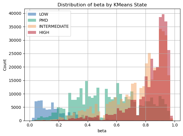
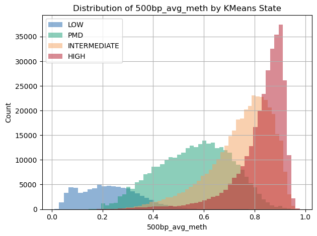
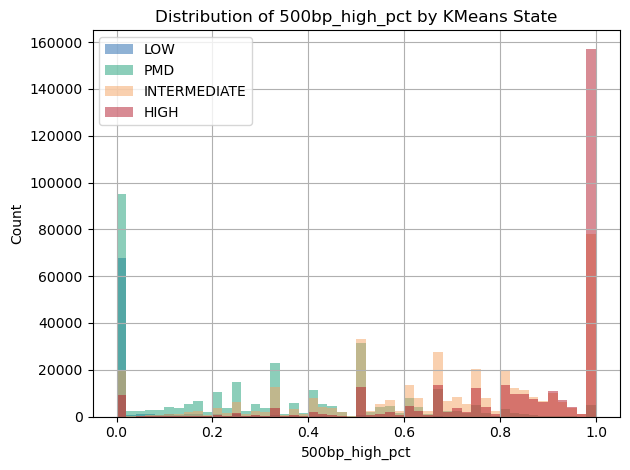
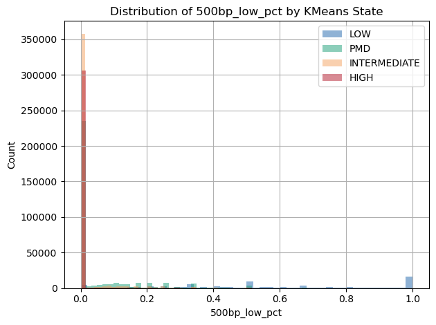
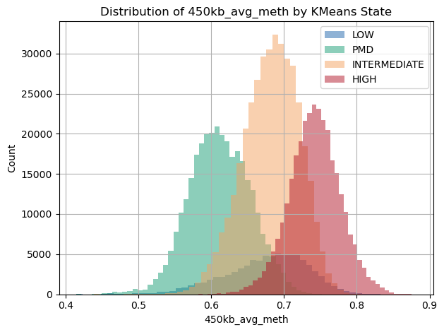
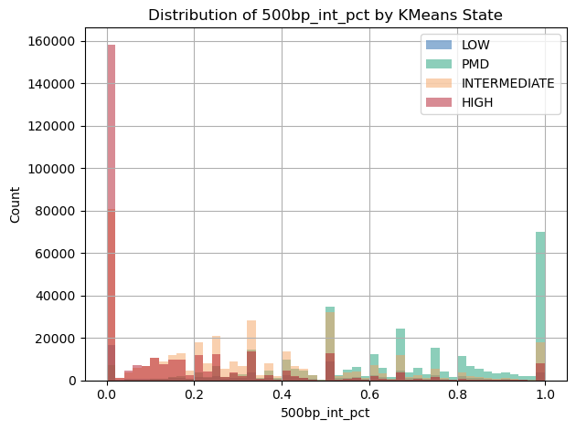
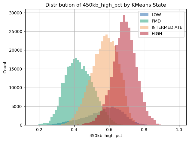
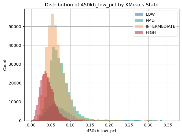
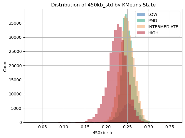
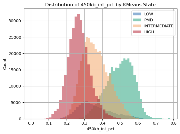
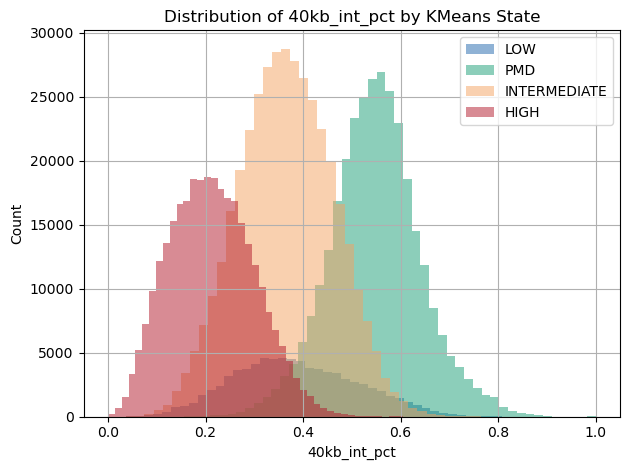
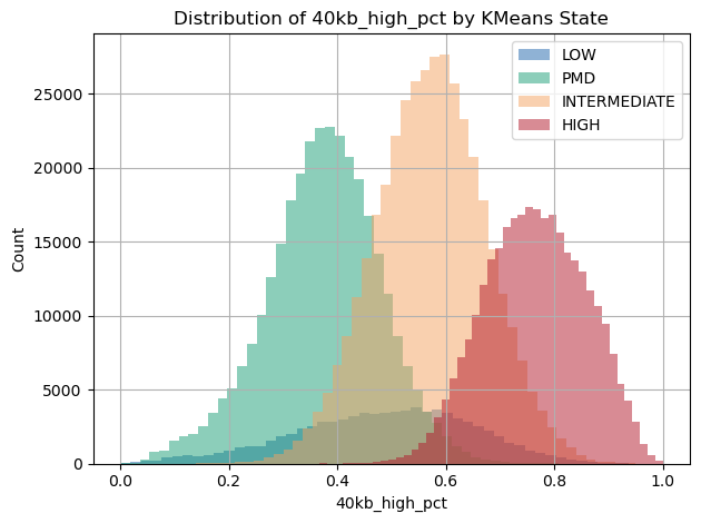
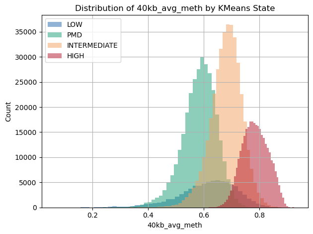
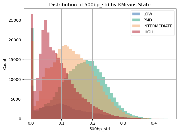
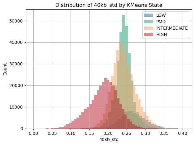
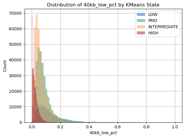
Feature distributions explain what each learned KMeans biological state represents in emission space. The histogram fills use the same STATE_COLORS mapping as the genomic and embedding plots, so the meaning of each color remains consistent throughout the gallery.

[21]:

model.assigner.plot_feature_distributions_by_kmeans_state(
    state_colors=STATE_COLORS
)

../../_images/tutorials_generated_07_plotting_examples_6_0.png

../../_images/tutorials_generated_07_plotting_examples_6_1.png

../../_images/tutorials_generated_07_plotting_examples_6_2.png

../../_images/tutorials_generated_07_plotting_examples_6_3.png

../../_images/tutorials_generated_07_plotting_examples_6_4.png

../../_images/tutorials_generated_07_plotting_examples_6_5.png

../../_images/tutorials_generated_07_plotting_examples_6_6.png

../../_images/tutorials_generated_07_plotting_examples_6_7.png

../../_images/tutorials_generated_07_plotting_examples_6_8.png

../../_images/tutorials_generated_07_plotting_examples_6_9.png

../../_images/tutorials_generated_07_plotting_examples_6_10.png

../../_images/tutorials_generated_07_plotting_examples_6_11.png

../../_images/tutorials_generated_07_plotting_examples_6_12.png

../../_images/tutorials_generated_07_plotting_examples_6_13.png

../../_images/tutorials_generated_07_plotting_examples_6_14.png

../../_images/tutorials_generated_07_plotting_examples_6_15.png

Comparing KMeans and rule-based assignments

This confusion-matrix view compares the learned KMeans labels with rule-based assignments for the prepared sample on the selected chromosome.

[22]:

model.analyzer.evaluate_clustering_concordance(
    sample_info=sample_info, chrom=PLOT_CHROM
)


Classification Report:
              precision    recall  f1-score   support

         LOW       0.61      0.72      0.66     80437
         PMD       0.79      0.52      0.63    316107
INTERMEDIATE       0.48      0.43      0.46    390073
        HIGH       0.47      0.66      0.55    313383

    accuracy                           0.55   1100000
   macro avg       0.59      0.58      0.57   1100000
weighted avg       0.57      0.55      0.55   1100000

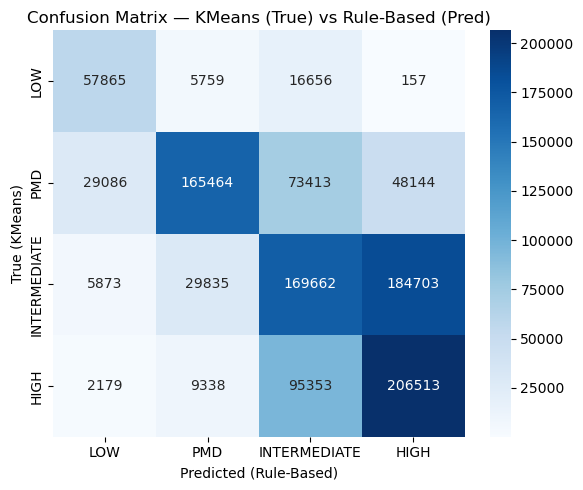
../../_images/tutorials_generated_07_plotting_examples_8_1.png

[22]:

	LOW	PMD	INTERMEDIATE	HIGH
LOW	57865	5759	16656	157
PMD	29086	165464	73413	48144
INTERMEDIATE	5873	29835	169662	184703
HIGH	2179	9338	95353	206513

Genomic label plots

Use model.assigner.plot_labels(...) when working directly with learned KMeans states. model.analyzer.plot_labels(...) can inspect KMeans and rule-based states with identical plot controls. For HMM states, use either the pathway convenience method, model.plot_labels(label_source="hmm", ...), or the underlying model.segmentor.plot_labels(...). Pass state_colors to use a project palette, sample_info_removed to show filtered probes, and max_points to bound browser rendering for dense samples. region_start and region_end zoom the displayed genomic window without changing the segmentation.

[23]:

fig = model.assigner.plot_labels(
    sample_info=sample_info,
    sample_info_removed=sample_info_removed,
    chrom=PLOT_CHROM,
    label_title="KMeans biological state",
    max_points=60_000,
    state_colors=STATE_COLORS,
)

[24]:

fig_kmeans = model.analyzer.plot_labels(
    label_source="kmeans",
    sample_info=sample_info,
    chrom=PLOT_CHROM,
    region_start=WINDOW_START,
    region_end=WINDOW_END,
    label_title="KMeans state for rule comparison",
    max_points=60_000,
    state_colors=STATE_COLORS,
)

fig_rule_based = model.analyzer.plot_labels(
    label_source="rule_based",
    sample_info=sample_info,
    chrom=PLOT_CHROM,
    region_start=WINDOW_START,
    region_end=WINDOW_END,
    label_title="Rule-based state in a genomic window",
    max_points=60_000,
    state_colors=STATE_COLORS,
)

[25]:

fig = model.plot_labels(
    label_source="hmm",
    sample_info=sample_info,
    sample_info_removed=sample_info_removed,
    chrom=PLOT_CHROM,
    region_start=WINDOW_START,
    region_end=WINDOW_END,
    label_title="HMM state in a genomic window",
    max_points=60_000,
    state_colors=STATE_COLORS,
)

[26]:

fig = model.segmentor.plot_labels(
    sample_info=sample_info,
    sample_info_removed=sample_info_removed,
    chrom=PLOT_CHROM,
    region_start=WINDOW_START,
    region_end=WINDOW_END,
    label_title="HMM state via MethylSegmentor",
    max_points=60_000,
    state_colors=STATE_COLORS,
)

Interval overlays

Cleaned-region overlays load previously generated calls.

[27]:

clean_summary_paths, clean_dir = model.get_clean_regions(
    regions_df=regions_chr1,
    sample_id=sample_info.sample_id,
    chrom=PLOT_CHROM,
)
clean_summary_paths, clean_dir

[27]:

({}, PosixPath('out/plotting_example_output/clean_regions'))

[28]:

fig = model.plot_labels(
    label_source="hmm",
    sample_info=sample_info,
    chrom=PLOT_CHROM,
    use_cleaned_regions=True,
    overlay_state="PMD",
    region_start=WINDOW_START,
    region_end=WINDOW_END,
    label_title="HMM state with cleaned PMD overlay",
    max_points=60_000,
    state_colors=STATE_COLORS,
)

Embedding plots

For a small number of points, use a scatter plot to inspect individual CpGs and PCA loading arrows. For dense data, use a hexbin plot and tune its grid size, minimum count, transparency, and border width. The genomic window arguments highlight overlapping CpGs in embedding space.

[ ]:

fig = model.plot_embedding(
    label_source="kmeans",
    sample_info=sample_info,
    chrom=PLOT_CHROM,
    method="pca",
    hexbin=False,
    include_biplot=True,
    include_metrics=True,
    label_title="KMeans state",
    region_start=WINDOW_START,
    region_end=WINDOW_END,
    region_chrom=PLOT_CHROM,
    state_colors=STATE_COLORS,
)

../../_images/tutorials_generated_07_plotting_examples_18_0.png

[34]:

fig = model.plot_embedding(
    label_source="hmm",
    sample_info=sample_info,
    chrom=PLOT_CHROM,
    method="pca",
    hexbin=True,
    hexbin_gridsize=80,
    hexbin_mincnt=25,
    hexbin_alpha=0.85,
    hexbin_linewidths=0.15,
    include_biplot=False,
    include_metrics=False,
    label_title="HMM state density",
    state_colors=STATE_COLORS,
)

../../_images/tutorials_generated_07_plotting_examples_19_0.png